
Google Sheets Formulas: How They Work and Essential Examples
If you’re working with data, you’re familiar with Google Sheets. But are you using it to the fullest? For most people, tasks like finding averages and counting thousands of cells would be a major headache — even mathematicians wouldn’t tackle them without a calculator. But Google Sheets’ formulas can handle these complicated tasks with ease. Whatever insights you need from your data, there’s probably a formula that’ll reveal them.
So forget about manually working with the data in your spreadsheets. Today, we’ll explain what Google Sheets formulas are, how to use them, and the essential Sheets formulas that will make your life easier.
What is a Google Sheets formula?
Formulas are like an advanced calculator built right into your spreadsheet. They let you go beyond just organizing your data, and use math to analyze it in different ways.
Any question you might have about your data can likely be answered with a formula.
- “How much did we spend on paper this month?”
- “Is anyone named Rosie enrolled at our school?”
- “What’s the average number of touchpoints it takes before a potential customer chooses to buy?”
Simple formulas include basic mathematical functions, like addition and subtraction. But there are also plenty of more complex queries and calculations, like finding an average or searching for a specific data point.
It would be painfully time-consuming to do all these calculations yourself — even simple ones like counting data points in a column. Plus, you’d be dealing with an unavoidable margin of human error.
That’s where Google Sheets Formulas come in. Once you’re armed with functions and formulas, working with data is faster and more accurate.
How to add Google Sheets formulas to your spreadsheet
Google gives you a few different ways to apply formulas to your data. All of them are easy and intuitive.
To choose formulas manually, enter an equals sign (=) into any cell on your sheet. Then, type in the formula you’d like to use, or select it from the Functions menu at the top right corner of the toolbar. Plug in the data you want to apply it to, hit Enter, and the result will display.
Here’s a super-basic Formula typed into a Worksheet.
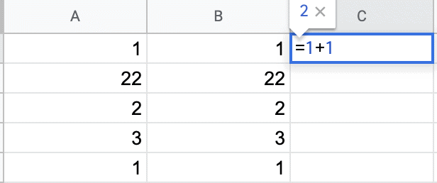
And here’s what it would look like if instead, you selected the formula from the Functions bar.

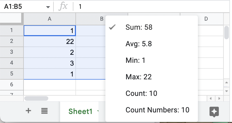
Google will also suggest the formulas it thinks you’ll find most useful. To try this method, select the cells you’d like to work with.
Google will automatically display a predicted formula (usually the sum) in the bottom right corner of your sheet. If you click on it, you’ll see other formulas you might want to use — and their results, all ready to go!
Here’s what that would look like in practice.

Applying formulas to cell addresses
Technically, you can use formulas like a calculator, applying them to actual values. But they’re much more useful when applied to specific cells, and whatever data they contain.
This might sound confusing, but it’s just a way to keep Formulas doing the work for you.
When formulas are applied to cells, they will automatically recalculate every time you change the data in them. That means the result stays accurate, even as you update the information in your Sheet.
This is called using a ‘cell reference.’
To do this, you’ll enter a ‘cell address’ into the formula instead of the data itself. A cell address is simply the row and column of the cell — for example, A1, F36, or DC612.
After typing =, you can type in the cell addresses, or just click on the cells themselves.
Here’s what the formula from above would look like, using cell references instead of integers.

Applying formulas to many cells at once
Google Sheets’ Fill function lets you apply that same formula to many different cells. Click on the bottom right corner of the cell and drag it outwards, over the other cells you’d like to apply it to.
Here, we’ve extended our simple addition formula downwards, to the rest of the rows in this sheet. As you can see, Google understands that we don’t just want to add 1+1 — we want to add up the numbers beside each other in these two columns.

The best Google Sheets formulas
Google Sheets offers hundreds of formulas that cover mathematics, finance, engineering, and even logic.
Here are a few of the most useful formulas (and types of formulas). We’ll start with some super common, indispensable types of formula, then finish off with a couple more advanced options that are no less handy.
As you get used to working with Sheets, you’ll likely come to rely on many of these.
You’ll see below that many of these formulas can be applied conditionally, so that Google Sheets only counts the cells that meet the criteria you decide. For example, you might decide only to apply a formula to values greater than 5, expressed as “<5”.
If you want to use one of these formulas (or any formula, generally) look it up here and get instructions directly from Google.
Basic Arithmetic
These are the simplest calculations you can perform in Google Sheets. You don’t even need a specific formula like the rest of the entries on this list — just use the below symbols to calculate right in your cell.
- Addition: =1+1
- Subtraction: =1-1
- Multiplication: =1*1
- Division: =1/1
- Exponents: =1^1
SUM
This handy formula lets you tally up a range of cells much more quickly than using the addition function.
As we mentioned, if you select a range of cells containing numbers, their sum will actually appear in the bottom right corner of your sheet.
- Basic sum formula: =SUM(A2:B2)
- Conditional sum, with one or multiple criteria =SUMIF and =SUMIFS
AVERAGE
If you’re working with numbers, this formula adds up all the selected cells and finds their average. It will discount any cells that are blank or don’t contain numbers.
- =AVERAGE(A2:B2): Find the average of a range of cells
- =AVERAGEIF and =AVERAGEIFS: Finds the average of cells that meet one or more criteria within your range
COUNT
If you want to know how many data points you’re working with, you don’t need to count them yourself. This formula does that for you, even if you’re working with a messy or incomplete spreadsheet.
- =COUNT: Counts how many cells contain numbers in your selected range
- =COUNTBLANK: Counts how many blank cells are in your range
- =COUNTA: Counts all the cells that have data in your range, both numbers and letters
- =COUNTUNIQUE: Discounts duplicate data. How many unique data points are in your range?
- =COUNTIF, =COUNTIFS: Counts how many cells in your range have data that meets certain criteria
MAX, MIN, and MEDIAN
If you’re wondering how large the range of numbers in your dataset is, these formulas will help you out. They’ll show you the highest, lowest, and middle value in your range.
- =MAX: Shows the highest number in your selected range
- =MIN: Shows the lowest number in your selected range
- =MEDIAN: Shows the number that’s closest to the middle of your selected range
VLOOKUP
Think of VLOOKUP as the search engine for Google Sheets formulas. It lets you look for data points in a sheet that fit certain parameters.
However, it only searches vertically — that’s the ‘V’ part. The key datapoint you’re looking for needs to be in a designated column, but it can bring you back a result that’s correlated to that point, even if it’s in a different column.
For example, you might search for the name of a student at your school (in one column), and ask VLOOKUP to tell you what grade she is in (from a separate column).
The formula looks a little confusing, but here’s how to use it. You can also get more detailed instructions on applying criteria to VLOOKUP directly from Google.
- =VLOOKUP(search_key, range, index, [is_sorted])
- “Search_key” is the datapoint you’re looking for
- “Range” is the range of cells you want to look through in the first column
- “Index” is the column the result you’re looking for is in
- “Is_sorted” is an optional field, where you tell Sheets if the column being searched has been sorted.
- Usually, you should enter “FALSE” into this field. Sheets will then search the whole range for an exact match to your search key.
- If you want to search instead for an approximate match, first sort the column you’re searching into ascending order. Then enter “TRUE”, or just leave this field blank.
IMPORTRANGE
This super handy formula lets you pull data from one spreadsheet into another — and if the original spreadsheet is updated, those changes will be reflected in the new sheet, too!
You’ll just need the URL of the spreadsheet you’re pulling data from, and the range of cells you want to bring in.
- =IMPORTRANGE(spreadsheet_url, [sheet_name!]range_string)
- “Spreadsheet_url” is the web address of the source spreadsheet. Enclose this in quotation marks.
- “Sheet_name!” is optional. It lets you bring in data from a certain sheet within the target spreadsheet, if it has multiple tabs, by entering that sheets name. If you omit this, Sheets will import data from the range you set in the first sheet.
- “Range_string” is the range of cells you want to import, like “C4:D16.” It should also be enclosed in quotation marks.
Need more info? Check out our dedicated Google Sheets importrange function guide.
Get more out of your Google Sheets with Unito
What if you could completely transform your Google Sheets with a single tool? Like building detailed, automated reports using data from other tools, streamlining data exports across databases, and more. That tool? Unito.
Unito is a no-code workflow management solution with some of the deepest two-way integrations for the most popular tools on the market, including Asana, Excel, Google Sheets, Jira, GitHub, and more. With a Unito flow, you can automatically export Jira issues to Excel, where they’ll be turned into rows. Then, whenever an issue is updated in Jira, you’ll see those updates in Microsoft Excel. No manual exporting required.
The best part? We built a template you can use to build automatic reports in Google Sheets from data in your project management tools. Get the template here.
Want to know more?
Check out how this Unito integration works, what you can sync with it, and more.
(Google Sheets) Formulas for success
Formulas are the key to getting value from Google Sheets. If you’re not using them, you’re missing out!
All those numbers and symbols can be intimidating at first, but there’s no reason to be scared. Formulas are just an efficient way to ask Sheets to do what it does best — work with data.