How to Use IMPORTRANGE in Google Sheets

• Unito home /
• Blog /
• How to Use IMPORTRANGE in Google Sheets

Published in Apps on 12/01/2024, last updated 03/03/2024.

It’s not uncommon for project managers to have multiple tabs open and flip between project boards, budgets, and timelines. There’s a lot of information to keep track of, and data is invaluable when it comes to determining performance targets and measuring success.

And, if you’re like me, you likely rely on Google Sheets to do a lot of math for you. Why waste time trying to crunch numbers when there are tools to calculate for you? There are countless Google Sheets formulas you can use. However, to use them successfully, you need to understand exactly what you need to do, and the best way to do it.

In this article we’re looking at the IMPORTRANGE function and how it can help you work faster and smarter.

What is IMPORTRANGE?

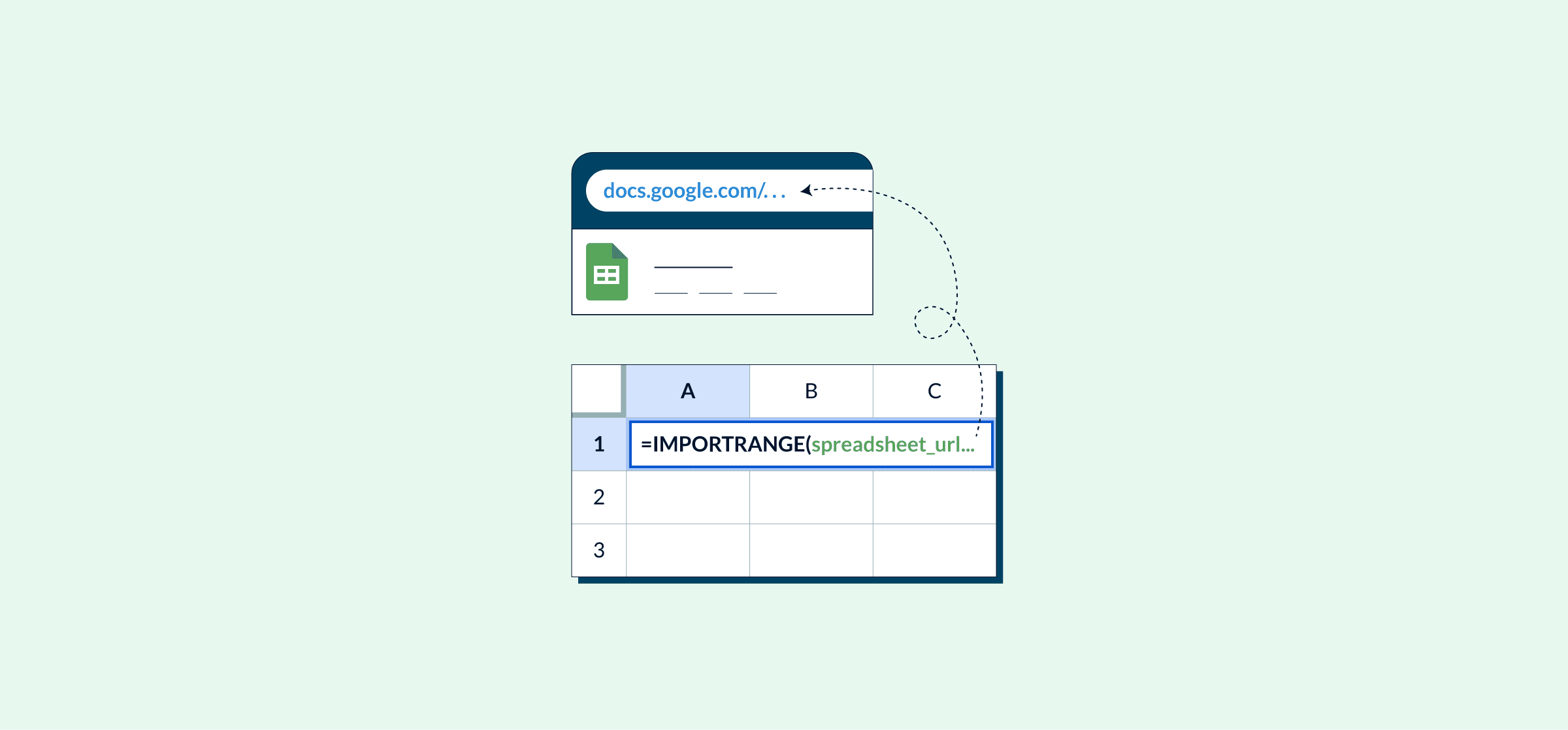
IMPORTRANGE is a function in Google Sheets (it does not exist in Excel) that allows you to import data from one spreadsheet to a destination sheet. That’s right, you can easily transfer data into one spreadsheet instead of flipping back and forth between multiple spreadsheets.

The syntax for IMPORTRANGE is: =IMPORTRANGE(spreadsheet_url, range_string)

• IMPORTRANGE: This is the specific function – importing a range of data.
• spreadsheet_url: This points to the URL of the spreadsheet where you’re importing data from.
• range_string: This specifies the range of data you’re importing.

4 steps to use IMPORTRANGE in Google Sheets

Before you begin, ensure you have access to each spreadsheet (check your permissions), and double-check the specific data ranges you want to import. Once everything is confirmed, follow these steps:

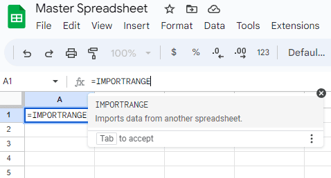
Step 1: Open your new spreadsheet and click in the top left cell – this is where the data will be imported to. To begin start typing the function =IMPORTRANGE (it will also appear in the drop-down menu of available functions, so you can select it from there too).

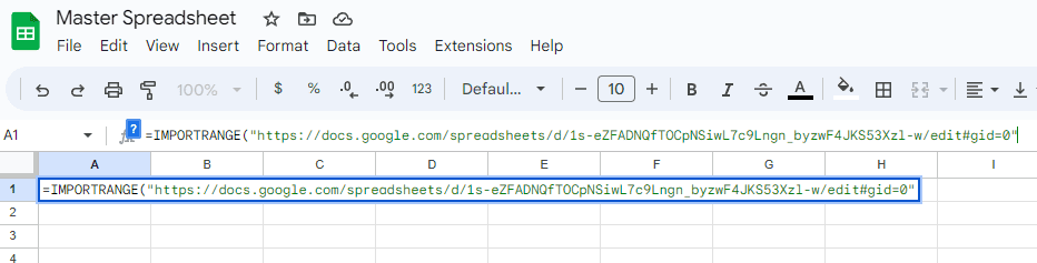
Step 2: Copy the full spreadsheet URL of the spreadsheet that you’re importing data from. If you want the formula to be shorter, you can copy just the spreadsheet key. Remember to keep the spreadsheet destination in quotations.

Full URL: https://docs.google.com/spreadsheets/d/1s-eZFADNQfTOCpNSiwL7c9Lngn_byzwF4JKS53Xzl-w/ 

Spreadsheet Key: 1DVwrdD3ZRzuT0zE5P_QChDbuvQ6_dWFL6j-eLoooMzE At this stage your formula would look like this: =IMPORTRANGE(“https://docs.google.com/spreadsheets/d/1s-eZFADNQfTOCpNSiwL7c9Lngn_byzwF4JKS53Xzl-w/”, range_string)

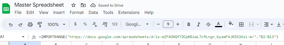
Step 3: Insert the range string — or cell range — for the data you want to import. This also needs to be in quotations. 

Example: “B2:B13” At this stage your formula would look like this: =IMPORTRANGE(“https://docs.google.com/spreadsheets/d/1s-eZFADNQfTOCpNSiwL7c9Lngn_byzwF4JKS53Xzl-w/”, “B2:B13”)

Step 4: Finish your formula by adding a closing parenthesis and hit enter. If this is the first time you’re importing data between the two sheets, you will get a #REF error like the one below.

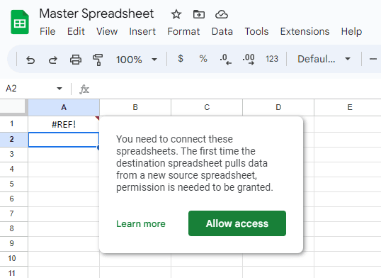
Click “Allow access” and your data will be imported.

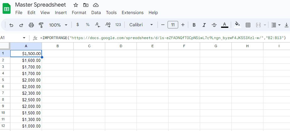
The import will happen immediately; there is no wait time, but if it’s a large amount of information it may take a few seconds. Now you can work with imported data from another spreadsheet. Better yet, all that data will update automatically — no extra manual work needed.

Common IMPORTRANGE errors

There are two common parse errors users come across when using IMPORTRANGE. Thankfully, both are easy to troubleshoot.

#ERROR!: This is the most common parse error and indicates an issue with the formula’s syntax. This includes forgetting quotations around ranges or missing a closing parenthesis, so double-check that everything is formatted properly. 

#REF!: As we mentioned above, you will see this parse error the first time you import data. If that’s the case a box will appear asking you to “Allow access” and once you click it, everything will load as expected. However, you will also see this if you try to manipulate or format any cells that you’re importing – you cannot do this with the IMPORTRANGE function. If that’s the case, delete your formula and redo it with everything as-is. If you want to format anything, you can’t use the IMPORTRANGE formula.

The benefits of using IMPORTRANGE

There are countless scenarios for when you should use the IMPORTRANGE function. When exactly should you use it? It really comes down to what type of work you’re doing, and how much time you want to save.

Some of the benefits of using IMPORTRANGE include: 

• You save time by streamlining data imports.
• It’s a quick and simple way to compare data. 
• You can easily import select rows of data from a larger private file to a shareable document without compromising information. 
• The function doesn’t require any browser extensions, Google Sheets integrations, or third-party apps to allow for data imports.
• There’s no equivalent function in Excel, so IMPORTRANGE is an invaluable tool to use exclusively in Google Sheets.
• You get results instantaneously. 
• It reduces the risk of human error.

When you don’t need to use IMPORTRANGE

IMPORTRANGE is designed to import data from one spreadsheet into another. That means there are two other common situations where you need to work with imported data and IMPORTRANGE isn’t the best solution.

Referencing data from somewhere else in the same spreadsheet

IMPORTRANGE will still let you pull data from one place in your spreadsheet to display somewhere else, but it’s not necessary. There’s actually a much simpler formula you can use. It’s called SheetName, and it lets you pull data from a specific range (or a single cell) in a spreadsheet, even if it’s from a different tab. Here’s the syntax:

• If you want data from a range: =’SheetName’![top-leftmost cell]:’SheetName’![bottom-rightmost cell]
• If you want data from a single cell: =’SheetName’!Cell

Working with imported data from other files

IMPORTRANGE only works with Google Sheets spreadsheets, but sometimes you need to bring in data from other sources. That’s where the IMPORTDATA function comes in. With this function, you can import data from CSV or TSV files, which are organized like spreadsheets. The syntax for this function is as follows:

IMPORTDATA(url)

Just plug the URL of the file you want to import data from in those brackets with quotation marks. Here’s an example, pulled right from Google’s support docs:

IMPORTDATA(“https://www2.census.gov/programs-surveys/popest/datasets/2010-2019/national/totals/nst-est2019-popchg2010_2019.csv”)

3 important Google Sheets functions to use alongside IMPORTRANGE

There are several other helpful formulas you can use in Google Sheets to improve your workflow when dealing with large amounts of. Let’s look at some of our favorites. 

COUNTIF

COUNTIF will show how many cells in a specific range meet the exact criteria you’re searching for. Instead of scrolling through rows and rows of data trying to find something, you can use this formula.

The syntax for COUNTIF is =COUNTIF(range, criterion)

You can use this to find sums above or below a certain amount: =COUNTIF(A1:A500, “<500”) 

Or, find cells containing specific text: =COUNTIF(B1:B50, “July”)

VLOOKUP

VLOOKUP is one of the most helpful formulas to use when sifting through data. You can use it to find information that’s related, such as a specific staff member and their salary, or the number of sales a specific team made in the month of September. In short, it easily compares data points.

The syntax for VLOOKUP is =VLOOKUP(search_key, range, index, [is_sorted])

SPLIT

The SPLIT function is great to use if you’re working with sheets full of text. It allows you to easily separate text based on a specific character or string and will fragment the results in separate cells in the same row.

The syntax for SPLIT is =SPLIT(text, delimiter, [split_by_each], [remove_empty_text])

Formulas in Google Sheets may seem overwhelming at first, especially if you’ve never used them before. However, they’re invaluable tools that you should get comfortable with.

Once you understand their power, you’ll be able to work much faster and smarter, and soon enough others will come asking you for help with their data sheets!

Want to do more?

Formulas are a great way to streamline your spreadsheets and make them do the heavy lifting. But Google Sheets has other built-in features that let you do even more; automations. In another guide, we break down how you can pull data from multiple Google Sheets and centralize it all in one place.

If you want to do even more, read Unito’s guide to automating Excel. Most of the tips can be applied to Google Sheets, too.

Google Sheets IMPORTRANGE FAQ

How can you use IMPORTRANGE in Google Sheets?

Using IMPORTRANGE in an empty spreadsheet can be done in just a few steps:

1. Open your spreadsheet and click the top-left cell.
2. Type in =IMPORTRANGE.
3. Open a parenthesis. Copy and paste the URL of the spreadsheet you want to import data from into the parenthesis. Make sure to put quotation marks around the URL.
4. Add a comma and insert the range string for the data you want to import (e.g. B2:B13) in quotation marks.
5. Add a closing parenthesis and hit Enter. Your formula’s done!

More of a visual learner? Here’s an example of what that formula looks like.

=IMPORTRANGE(“https://docs.google.com/spreadsheets/d/2s-eZOADNXfTODpNSiwL3c0Lngn_byzwF4JKS53Xzl-w/”, “B2:B13”)

What’s the difference between IMPORTRANGE and IMPORTDATA?

While both of these formulas allow you to import data into your spreadsheets, they have one key difference.

IMPORTRANGE lets you import a range of data from one Google Sheets spreadsheet into another. IMPORTDATA lets you transfer data from different file types (e.g. XML, HTML, CSV) to your spreadsheet. So while they both let you import data, they’re for completely different sources.

How do you use IMPORTRANGE in Excel?

The IMPORTRANGE function doesn’t exist in Excel. That said, there are two ways to replicate it, depending on which version of Excel you’re using (Excel Online or the desktop version).

• If you’re using Excel Online, you can use the Workbook Links feature to essentially replicate IMPORTRANGE in your spreadsheets.
• In Excel desktop, you can use Paste Link to import data from another Excel spreadsheet (or even multiple spreadsheets).