How to Create Pivot Tables in Google Sheets
Pivot tables are an invaluable tool that can be used in both Google Sheets and Excel. They’re a great way to represent data in a visual way, and they’re not as hard to set up as you might think.
If you’ve never played around with them before it’s time to learn. In this article, you’ll learn exactly what a pivot table is, what they’re commonly used for, and how to create them in a few simple steps.
What is a pivot table?
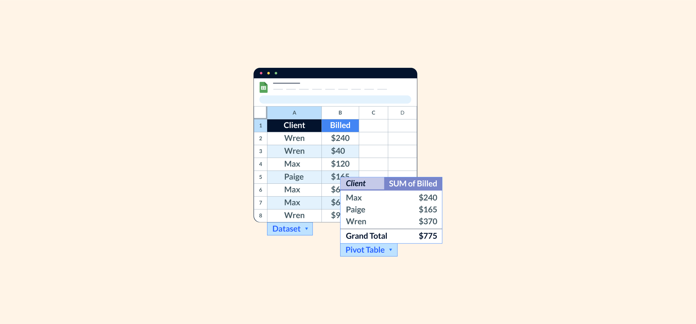
A pivot table is a tool that’s often used to help summarize large amounts of data. You can dynamically change the way data is presented, incorporate functions, and filter, sort, or rearrange how everything is displayed. Pivot tables are another way to create visuals, like charts or graphs, which can help highlight trends.
When creating pivot tables, you literally “pivot” your data by rearranging it, hence the name. This allows you to easily view data in different ways, highlighting trends or providing new insights you might’ve missed before.
Pivot tables are secret weapons for people who live and breathe spreadsheets. Knowing how to use them will allow you to manipulate data and analyze it easily.
What are pivot tables for?
There are countless ways to use pivot tables to help break down your data. You can use them for the following:
- Comparing data. You can easily break out sets of data in a pivot table to quickly compare information. Need to put Q1 and Q2 sales next to each other for a high-level overview, with a breakdown by team members? Use a pivot table.
- Highlighting trends and patterns. If your team’s sales for a specific month are thrown into a sheet, it’s hard to see who met or exceeded their goals and who didn’t. A pivot table will help you find sales patterns and see who the top (and lowest) performers are.
- Planning future goals and milestones. Pivot tables can help you easily compare historical data against present-day data — seeing how everything grows or declines will help set realistic goals for your team to work towards.
- Formatting and cleaning up data. When you work with large sheets of data there will likely be duplicates, misspellings, or other mistakes due to human error. Pivot tables will help you find these and clean them up, ensuring all your information is correct. You can also group or combine sets of data to make formatting a breeze.
Before you start creating pivot tables you should know what your end goal is. There are lots of ways to manipulate your data, so knowing exactly what you’re looking for will help. However, if you’re new to using pivot tables, take some time to play around with them and learn what you can do.
How to create a pivot table in Google Sheets
Step 1: Enter and format your data
You’ll need to have all your data in a spreadsheet to create a pivot table. If you have data in multiple places, use the IMPORTRANGE function to transfer everything to one sheet.
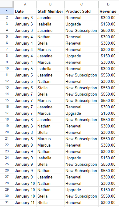
Below you can see the data we’ll be using for this step-by-step guide. In this example, we’ll be looking at sales by team members throughout the first eleven days of January.
Step 2: Insert your pivot table
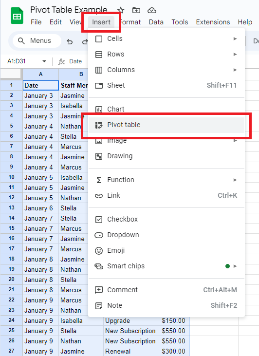
To insert your pivot table, begin by highlighting all the data you want to include (we’ve selected A1:D31 from the example above). Then, click “Insert” in the top menu, and select “Pivot table.”
You’ll get a prompt to enter your pivot table in a new sheet or the existing one. Where you insert it is up to you. For this example, we’ll keep working in the same sheet.
Step 3: Customize your pivot table
Once you’ve inserted your pivot table, you’ll be able to see the “Pivot table editor” on the right-hand side. This tool will help you customize your data to suit your needs.
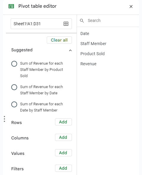
There are suggestions for ways to format data, but you can also create your own depending on what you need. Clicking through the suggested options first will give you a sense of how your data can be presented.
Here’s how we customized our pivot table:
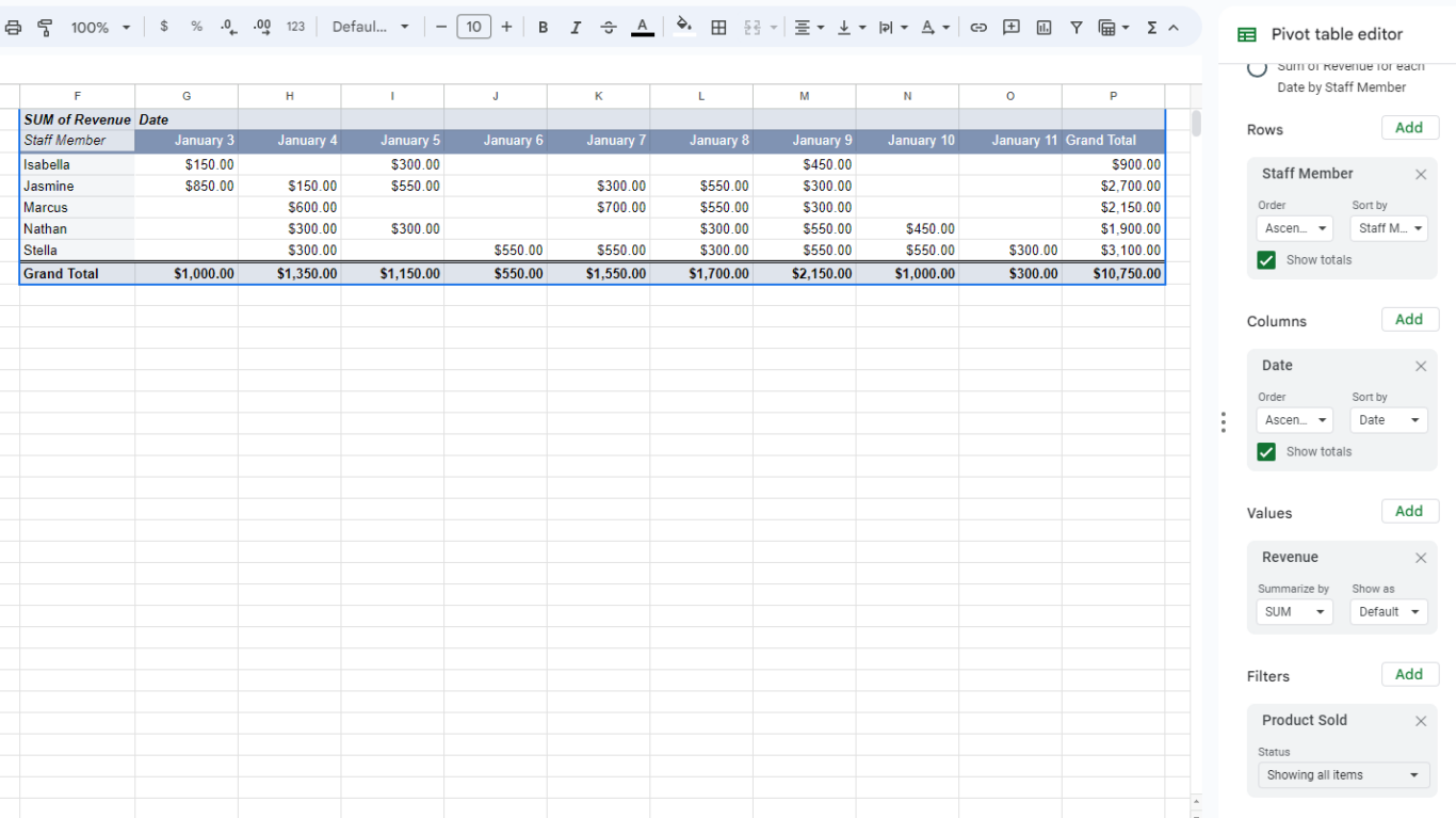
Now we can easily see sales per day by team members, with revenue totals along the bottom row. Currently, it shows total sales, but we also added a filter so we can toggle between different products. This makes it easy to break out new subscriptions, renewals, and upgrades.
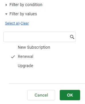
If you want to filter for only one value, simply edit that option.
Depending on how much data you have your rows, columns, values, and filters will look different. You may need to include all of them, or only a handful, depending on your needs.
Switching things around is simple: drag and drop them in the pivot table editor or select new options from the drop-down menu.
And that’s it! Now you know how to create pivot tables in Google Sheets.
How to create a pivot table in Excel
Creating pivot tables in Excel is very similar to Google Sheets. For this guide, we’ll use the same data from our previous example.
Step 1: Enter and format your data
You’ll need to have all your data entered and formatted in your sheet to begin. If you’re working with multiple sheets, pull all your data into one sheet before starting.
Step 2: Inset your pivot table
To insert your pivot table, start by highlighting all the data you want included. Then, click the “Insert” option in the top menu, and select “PivotTable.”
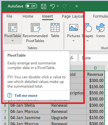
If you click the image — rather than the word “PivotTable” — you’ll be prompted to specify the table range. These are the cells we’ve already highlighted, but you can adjust them if needed. Then, you can specify where to insert the pivot table, either in the same sheet or a new one.
If you select the bottom half of the button — the text and down arrow only — you can choose to use data either “from table/range” or “from external data source.” In this article, we’ve been using data from our own sheets but depending on your work, you may need to sync with external sources.
We’ll continue with data from our table/range and insert it in the same sheet.
Step 3: Customize your pivot table
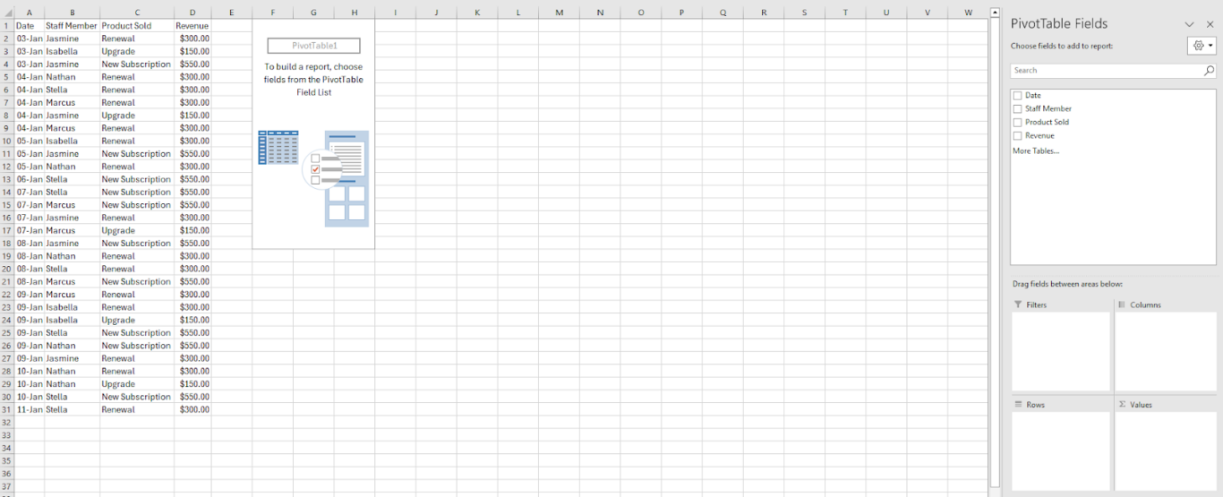
Once your pivot table is inserted it will appear blank on your sheet, but the editor tool will show up on the right-hand side. In Excel, it’s labeled as “PivotTable Fields” and is a little different from Google Sheets.
Unlike Google Sheets, there aren’t suggested formats or views. In Excel, you’ll have to create your own pivot table setups. Here’s how we created ours (with additional formatting to show dollar amounts):
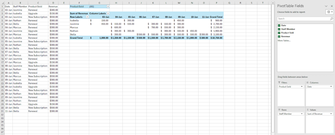
Formatting a pivot table can seem overwhelming if you’ve never done it before. It’s best to understand what each field refers to so you can easily arrange your data.
- Filters: Filters are optional and often used to highlight specific data. Using them will allow you to organize your data easily and apply restrictions to what’s being shown. In our example we filter by product sold to further isolate sales data.
- Column: Data selected for columns will appear across the top of your pivot table. In our example we put dates here to easily see and analyze data over time.
- Rows: Data selected for rows will appear down the first column, like a Y-axis on a chart or graph. Here we have team members in rows so we can easily see a breakdown of their individual sales by day.
- Values: Values refer to the specific data being measured and summarized. In our example we put revenue here since that’s what we want to measure.
Once your pivot table is created you can format it with different colors or fonts, pull in additional values, apply filters, and more. All of this will depend on your specific needs.
And there you have it – now you can create pivot tables in Excel and Google Sheets!