
How to Use Conditional Formatting in Your Spreadsheets
Staring at columns and rows of raw data can be draining. After a while, all the numbers blend together, and you don’t remember what you’re looking for anymore. If this sounds too familiar, then you might need to start using conditional formatting rules in your spreadsheets. It will help you find the information you’re looking for quickly, and you’ll be able to sort through data like a pro.
In this article, we’ll look specifically at how to use conditional formatting in Microsoft Excel, but will include tips for users who prefer Google Sheets as well.
What is conditional formatting?
Conditional formatting is a feature that you can find on Excel’s “Home” tab that allows you to format rows and columns of data to highlight specific information. If you’re using Google Sheets, you can find the feature under the “Format” tab.
It allows you to use preset conditions (or rules, as they’re often called). Or, if you’re feeling creative, you can create your own rules for more advanced use. When you apply conditional formatting to a cell, the background and/or text color will change.
Conditional formatting operates using an if/then statement, much like other formulas in Excel: if the value of the cell matches the condition you’ve set, then the cell will be formatted with a new color.
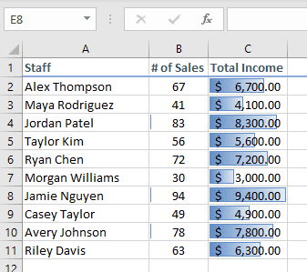
Let’s take a look using a simple example. In this spreadsheet, we want to see all employees who made more than 60 sales in the past month, so I’ve applied a conditional formatting rule to highlight every cell starting at 60 and above.
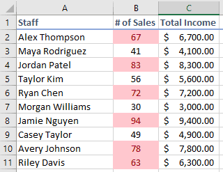
Now, it’s easy to see who met the monthly sales goals, and who is lagging.
How to apply conditional formatting
Applying conditional formatting might sound intimidating, but it’s actually pretty simple.
4 Steps to applying conditional formatting in Excel
Let’s review the steps using the example provided above to see how I was able to highlight employees who hit their sales target in Excel.
Step 1: Get your data ready
First, you need to have all your data organized in a spreadsheet. Know ahead of time what row or column you want to manipulate, and what information you’re looking for. For this example, we’ll use the spreadsheet shown above illustrating employees, number of sales, and total income made.
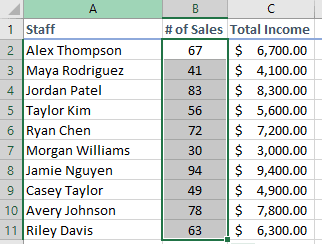
Step 2: Select a range
Next, highlight or select the range you want to apply a conditional formatting rule to. In this example, we’ve selected all of column B.
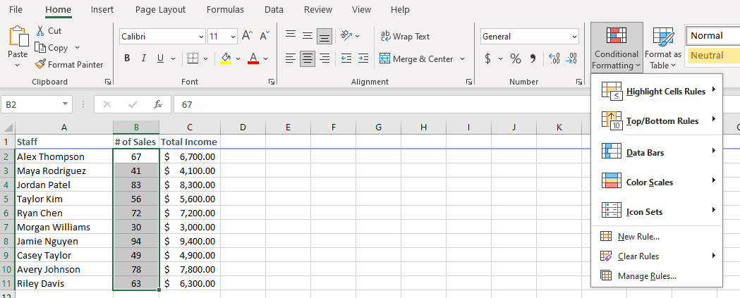
Step 3: Choose what conditional formatting rule you want to apply
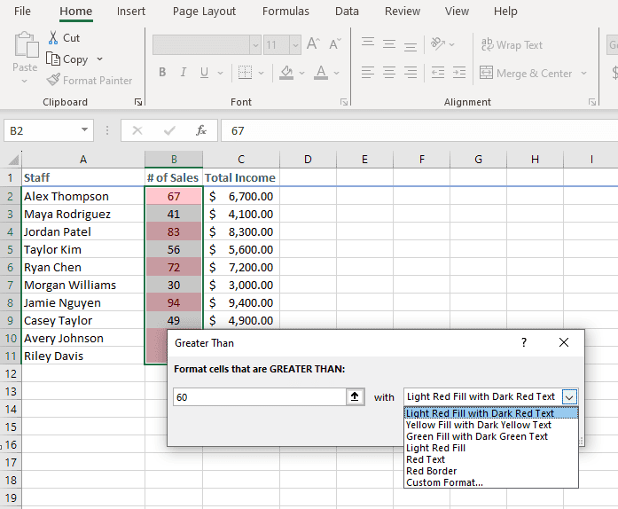
Then, click on the “Conditional Formatting” button under the “Home” tab and select the rule you want to apply. For this example, we’re using “Highlight Cell Rules.”
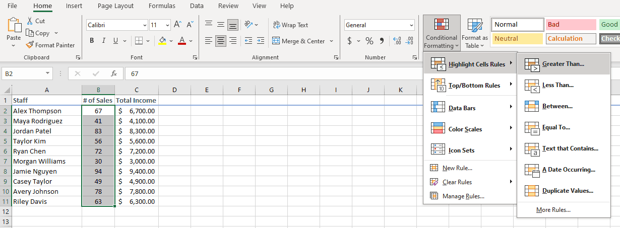
Then, select “Greater Than…” since we’re looking specifically for numbers greater than our target (60).
Step 4: Define the specifics of the rule
Next, you need to set the rules. In this case, it will ask for a number to begin sorting with (remember, we want 60 or higher). Then, you need to select how these cells will be formatted; the default “light red fill with dark red text” works.
Once that’s set, hit “OK” and you’re done!
You’ve successfully applied a conditional formatting rule in Excel to display all cells in this column with numbers 60 or greater with a red background and text. Finding this information is quick and easy now since it stands out drastically from the rest of the data.
Now we’ll do the same thing in Google Sheets.
4 steps to apply conditional formatting in Google Sheets
For this breakdown we’re going to assume you already have your data ready and are all set to begin formatting it.
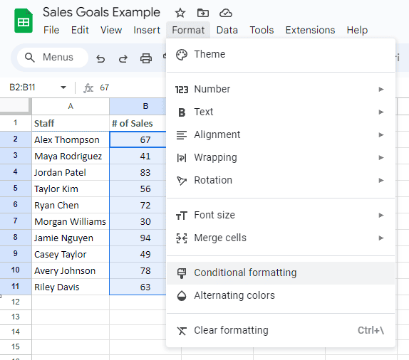
Step 1: Find and select “Conditional Formatting”
Remember, in Google Sheets you’ll find this feature under the “Format” tab along the top of your sheet.
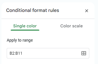
Once you click on this option, it will open a tab on the right-hand side of your sheet called “Conditional format rules.”
Step 2: Select your range
In this tab you can select the range you want to apply the formatting to under “Apply to range” – we’ve already selected B2:B11, but you can edit your selection if needed.
Step 3: Select your format rule
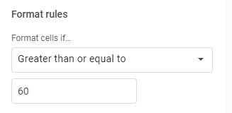
Then, click on the drop-down option for “Format rules” to select what you want. There are a lot of options in Google Sheets, from date formats to dropdown lists, but for this example, we’re looking for “Greater than or equal to.”
Step 4: Input your value
Then, you can input the value you want to focus on (we’ve used 60 again).
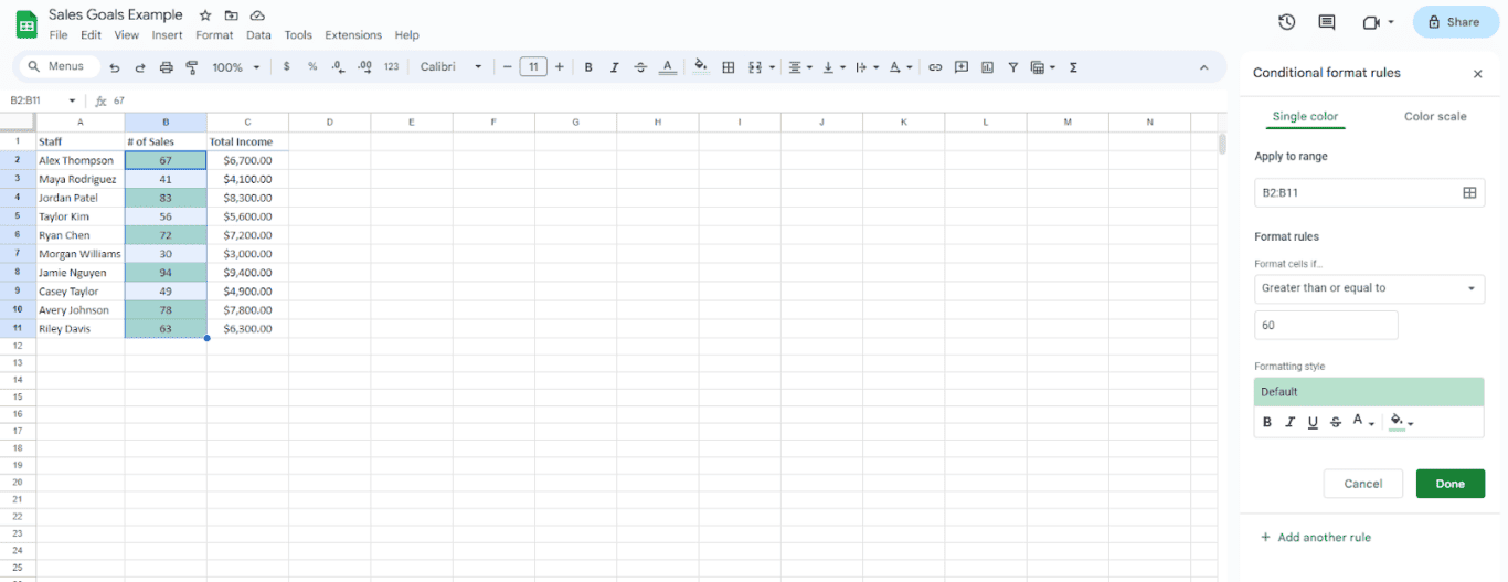
Once you enter a value, Google Sheets will automatically apply the conditional formatting rule using the default formatting style, green. You can click through those options to stylize it however you want.
That’s it – you’ve successfully applied a conditional formatting rule in Google Sheets!
How to clear conditional formatting rules
If you’ve applied a bunch of conditional formatting rules and no longer want them, it’s easy to reset your data.
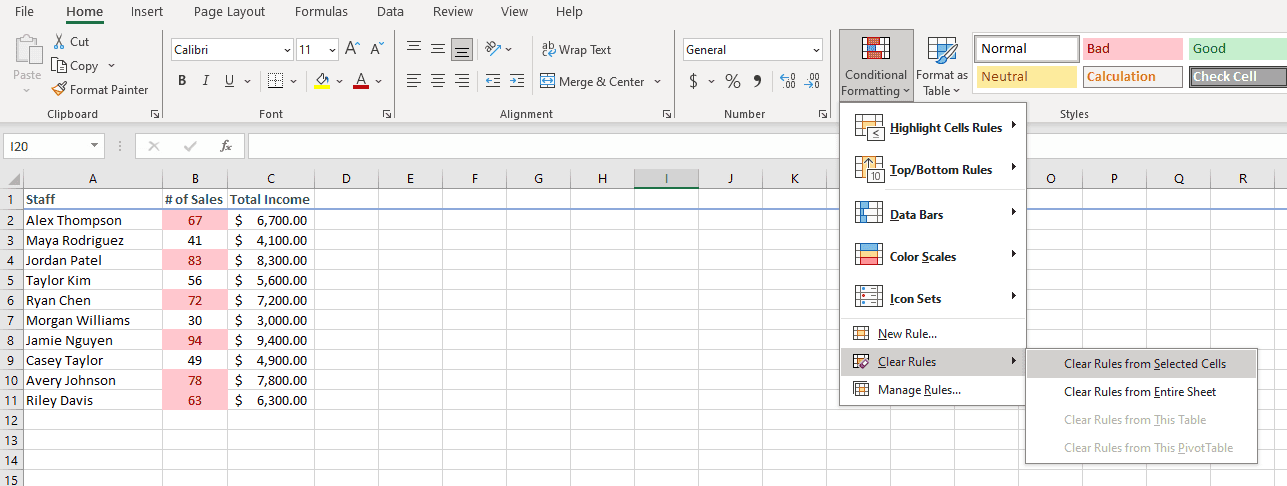
In Excel, select the “Conditional Formatting” button again, and hover over “Clear Rules” – you can choose to clear rules from the specific cells you currently have selected, or from the entire sheet.
In Google Sheets, the list of rules you’ve applied will show up on the right-hand side whenever you select “Conditional formatting” from the “Format” tab. If you hover over the rule, a trash bin icon will appear. Click on it to remove that specific rule from your sheet.

Types of conditional formatting in Excel
There are different types of conditional formatting you can use in Excel, and each one is incredibly useful.
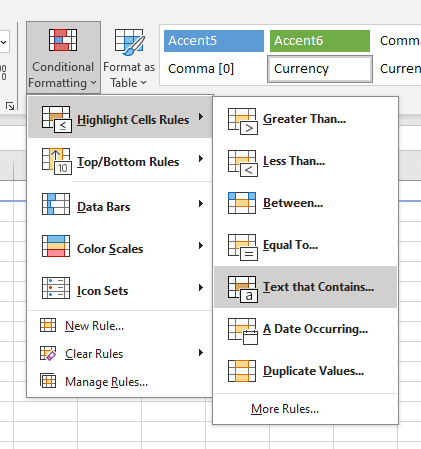
Need to highlight data related to a specific team member? Select “Conditional Formatting” > “Highlight Cell Rules” > “Text That Contains.” Bam, everything in the range you’ve selected containing those words is now highlighted.
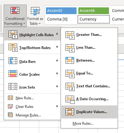
Trying to find duplicate information? Highlight your range, select “Conditional Formatting” > “Highlight Cell Rules” > “Duplicate Values.” No more going cross-eyed trying to manually pick out doubles. This option also lets you choose between duplicate or unique values, so you can quickly find either depending on your needs.
Under “Top/Bottom Rules” you’ll also find options to highlight data related to percentages and averages.
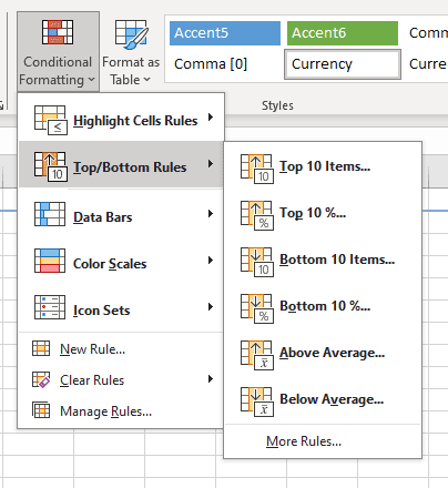
These rules will help you easily find the top performers on your team or highlight budget lines that are trending above or below expectations. There’s no reason to manually do the math yourself because these conditional formatting rules will immediately highlight the cells you’re looking for; you just need to know exactly what you want to find in your spreadsheets and input the appropriate metrics when setting up your rules. Knowing what you’re looking for is key.
Using “Data Bars,” “Color Sets,” and “Icons” refer to different ways that your cells will be styled. Typically, the colours will relate to the values, and how high or low they are compared to everything else in the selected range.
In the example below, you can see how I’ve applied “Data Bars” to illustrate how close each team member came to meeting their sales goal: the closer their total was to the goal, the more filled in the cell is.
How you use these style options will depend on your personal needs and whether you want to add more detail to your reports. It also helps add a visual component, which can make the data easier to read for people who don’t deal with numbers too often.
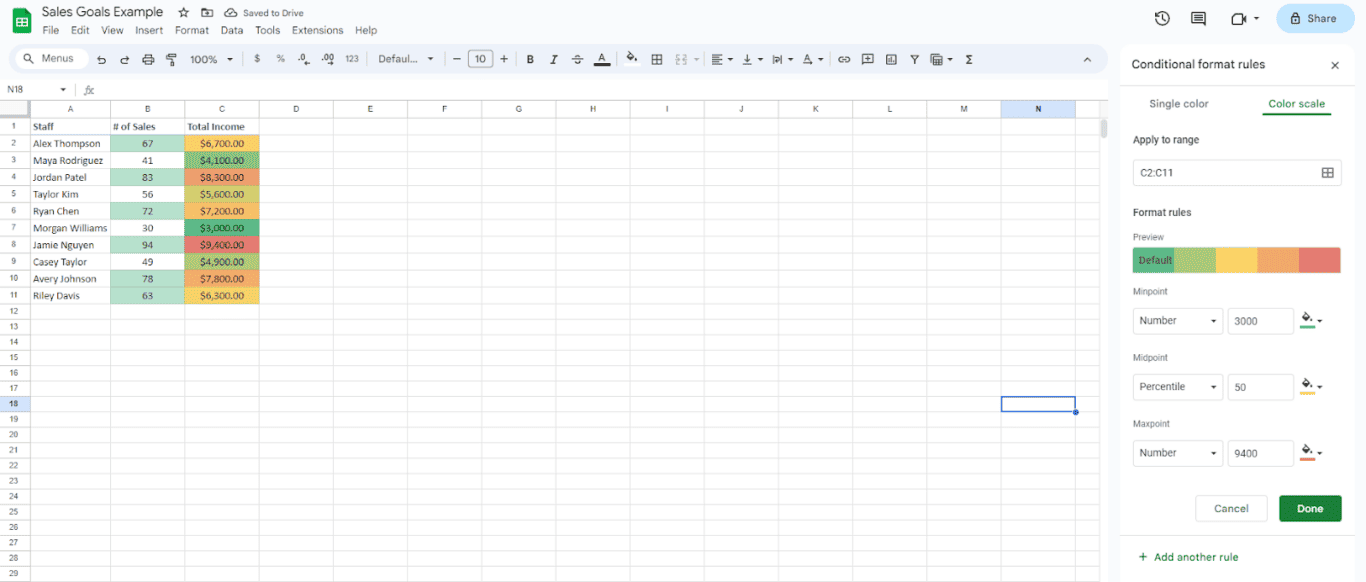
Conditional formatting styles in Google Sheets
For those using Google Sheets instead of Excel, there are different options available for styling your data.
When you set up a conditional formatting rule, you can switch between “Single color” and “Color scale” when setting up the rule. If you select “Color scale” you’re presented with options: you can swap out the default green for a different color, set minimum and maximum values for when the color should change, and select the ranges to apply everything to.
Benefits of conditional formatting
Whether you use conditional formatting in Excel or Google Sheets, you’ll benefit from the following:
- Data is easier to read. With conditional formatting rules applied, you can quickly skim through your spreadsheet and find exactly what you’re looking for without getting distracted by all the other rows and columns of information.
- You can highlight trends. Looking for sales leads who are consistently top performers? Apply a rule top/bottom rule to see who always comes out on top, month over month, instead of shifting through different sheets of data.
- Validate data inputs. Worried about duplicate cells or misspellings? Conditional formatting allows you to easily find and fix these issues.
- Customize your spreadsheets. Have you ever been jealous of other spreadsheets that are color-coded and customized to perfection? It’s because whoever made them is a master of conditional formatting rules, and now you are too!
Shifting through data just got a whole lot easier for you, so there’s no need to stress over your next report. Instead, harness the power of conditional formatting and let your data speak for itself!